Geographical maps can often be usefully represented as simple graphs. In one representation that comes to mind immediately, vertices correspond to countries or states and there is an undirected edge between two vertices if the corresponding states share a common border.
Basic graph algorithms can then the applied to identify reachability via land routes, the number of hops involved in such route and so on. Each hop corresponds to a move from one state to a neighboring one. If the map contains disconnected entities, the connected components can also be identified.
In this post, the contiguous-usa dataset from Knuth’s page is used to identify the number of hops between a starting state in the US and all other states in the US mainland. This dataset covers the connected US mainland only and thus excludes Hawaii and Alaska which are not physically contiguous to other states.
The next post deals with the world map using of the Correlates of War Contiguity dataset and identifies connected components i.e. sets of countries that are connected to each other by a land or river border. Some countries themselves contain territories physically disconnected by sea but they have been treated as a single entity for simplicity.
Overall, these posts illustrate how raw datasets can be represented as graphs, how basic algorithms can be applied to them and how the results can be presented in a simple visual way in web applications. These ideas can be expanded to complex graphs that sophisticated applications have to work with, and more complex visualizations can also be built by extending these concepts.
Shown below are the initial 7 lines and the last 7 lines from contiguous-usa.dat. Each line in the file represents an edge (u,v) i.e. a border between two states. If (u,v) is present in the file, (v,u) is not.
> head -7 contiguous-usa.dat
AL FL
AL GA
AL MS
AL TN
AR LA
AR MO
AR MS
> tail -7 contiguous-usa.dat
OK TX
OR WA
PA WV
SD WY
TN VA
UT WY
VA WV
The number of edges and vertices can be found as shown below. These are some initial, exploratory checks on the data.
> wc -l contiguous-usa.dat
107 contiguous-usa.dat
> awk '{print $1; print $2}' contiguous-usa.dat | paste | sort | uniq | wc -l
49
Looking into the data in more detail, it is seen that the 49 is due to the inclusion of DC as a state. The US has 50 states excluding DC. Here DC is included while Alaska (AK) and Hawaii (HI) are not.
The contiguous-usa.dat file is read by a Python program graphProcessor.py and converted internally into a dict-based adjacency list representation where the keys are the nodes and the value for each key is a list of nodes (states) that have edges with that node. The edges are undirected - so for each edge (u,v) in the file, v is present in u’s list and u is present in v’s list.
This graph does not have weights on its edges but that could be incorporated easily by having (vertex,weight) tuples in the lists instead of just the vertices. And if the edges were directed, then for edge (u,v), v would be in u’s list but u would not be in v’s list. The textual form of the adjacency list representation, as generated internally by the program, is available here. The first field is a vertex and the remaining fields are the neighbors of the vertex.
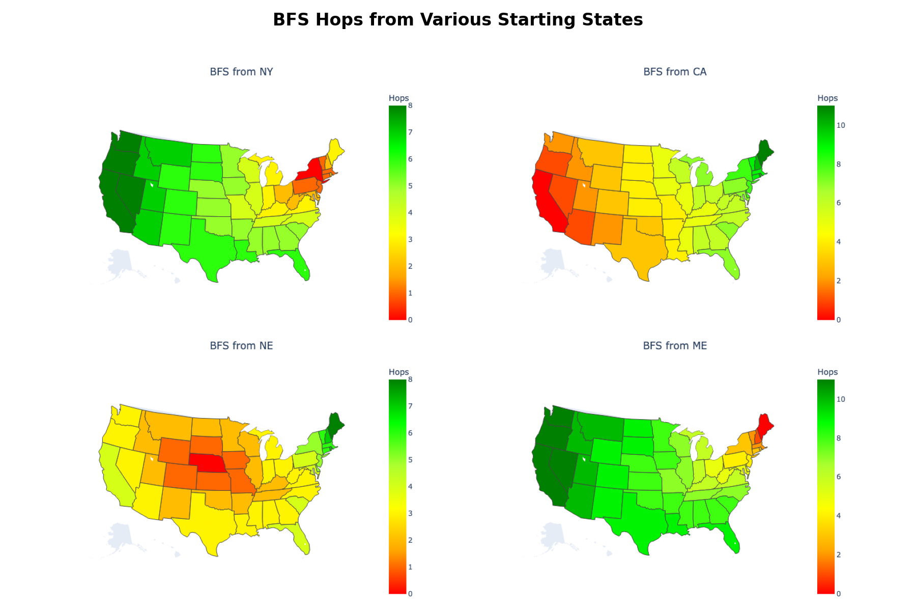
A Breadth First Search is run from four states NY, NE, CA and ME which are located to the east, center, west and far north-east respectively. The results are shown below as static screenshots.
The interactive view is available here
A separate color is used for the number of hops from the starting vertex, with red being used for a hop count of 0 i.e. the starting vertex.
The results show that the maximum number of hops is different for different starting vertices. One of the reasons is the nature of connectivity of the states in the far north-east. Starting from CA, there is a maximum of 11 hops as compared to starting from NY or NE when a maximum of 8 hops is seen.
Another interesting thing is observed when we compare the visual for CA with that for ME as the starting vertex. When starting from CA, ME is the only state at a distance of the 11 hops. But when starting from ME, several states on the west are at a distance of 11 hops. On further analysis, other insights of a similar nature can be obtained.