Aim

A projectile is launched with velocity \(v_0\) at an angle θ to the horizontal. We want to investigate and analyze its trajectory and study the effect of changing the launch angle θ. We illustrate it visually for a clearer understanding.

1. Maximum Height

For finding maximum height \(h\) reached by the projectile, we consider motion in vertical direction i.e. along y-axis.

Initial velocity = \(v_0sinθ\)
Final velocity = \(0\)
Acceleration = \(-g\)

Using
\[ v^2 - u^2 = 2as \]

we get
\[ 0^2 - v_0^2sin^2θ = 2(-g)h \]

\[ v_0^2sin^2θ = 2gh \]

i.e.

\[\begin{align} \Large h = \frac{v_0^2sin^2θ}{2g} \end{align}\]

2. Time of Flight

For finding maximum height \(h\), we again consider motion in vertical direction.

initial velocity = \(v_0sinθ\)
displacement = \(0\)
acceleration = \(-g\)

Using

\[ s = ut + \frac{1}{2} at^2 \]
we get

\[ 0 = v_0tsinθ - \frac{1}{2}gt^2 \]

\[ 0 = t(v_0sinθ - \frac{1}{2}gt) \]

This gives either \(t = 0\) (not the valid root we need) or

\[ v_0sinθ - \frac{1}{2}gt = 0 \]

Thus, the time of flight is as below :-

\[\Large t = \frac{2v_0sinθ}{g}\]

3. Range

For finding the range \(s\) or the distance where the projectile lands on the ground, we consider motion in horizontal direction i.e. along x-axis.

Initial Velocity = \(v_0cosθ\)

Time of Flight = \(\Large \frac{2v_0sinθ}{g}\) (from section 2)

\[ s = ut \]

\[ = \frac{(v_0cosθ)(2v_0sinθ)}{g} \]

\[ = \frac{2v_0^2sinθcosθ}{g} \]

\[ = \frac{v_0^2sin2θ}{g} \]

i.e.

\[\Large s = \frac{v_0^2sin2θ}{g}\]

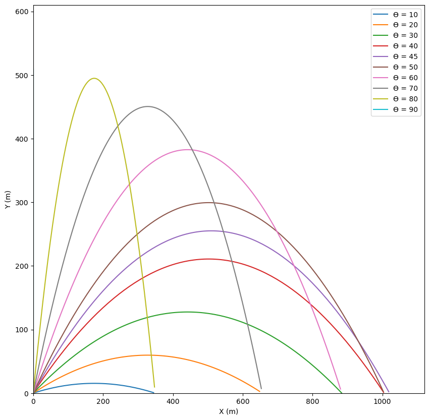
4. Visual Plots

Using the equations derived in sections 1, 2 and 3, we can compute the trajectory of the projectile and plot it.

Using time as the independent variable, we generate \(x\) and \(y\) and plot \(y\) versus \(x\) for a range of values of \(\theta\) from \(10^{\circ}\) to \(90^{\circ}\). We use \(g = 9.8 m/s^2\) and \(v_0 = 100 m/s\)

Code

# Compute points

def plot_trajectory(theta):
    theta_rad = (theta * math.pi) / 180
    x = []
    y = []
    t = 0
    t_step = 0.1
    t_flight = (2 * V * math.sin(theta_rad)) / g

    while t < t_flight:
        x_t = V * t * math.cos(theta_rad)
        y_t = V * t * math.sin(theta_rad) - 0.5 * g * t * t
        #print("t=%.2f x=%.2f y = %.2f" % (t, x_t, y_t))
        x.append(x_t)
        y.append(y_t)
        t = t + t_step
    plt.plot(x, y, label='ϴ = ' + str(theta))

# Constants    
g = 9.8
V = 100

# Plot
x_lim = V*V/g + 100
y_lim = V*V/(2*g) + 100

fig, ax = plt.subplots(1, figsize=(10,10))

ax.set_xlim(0, x_lim)
ax.set_ylim(0, y_lim)
ax.set_xlabel("X (m)")
ax.set_ylabel("Y (m)")

theta_list = [10, 20, 30, 40, 45, 50, 60, 70, 80, 90]
for theta in theta_list:
    plot_trajectory(theta)

_ = ax.legend(loc="upper right")

5. Animation of Trajectory

Finally, we animate the trajectory of the projectile for a certain value of \(\theta = 45^{\circ}\). It is easy to change \({\theta}\) and run the animation for various other values of \({\theta}\)

Code

# Compute points

def compute_trajectory(v, theta, x, y, num_points):
    theta_rad = theta * math.pi / 180

    t_flight = (2 * v * math.sin(theta_rad)) / g

    num_points = 100
    
    t_step = (t_flight/num_points)
    t = 0          
    while t < t_flight:
        x_t = v * t * math.cos(theta_rad)
        y_t = v * t * math.sin(theta_rad) - 0.5 * g * t * t
        #print("t=%.2f x=%.2f y = %.2f" % (t, x_t, y_t))
        x.append(x_t)
        y.append(y_t)
        t = t + t_step
        
    return t_flight